Vertical Federated Learning example#

This example will showcase how you can perform Vertical Federated Learning using Flower. We’ll be using the Titanic dataset to train simple regression models for binary classification. We will go into more details below, but the main idea of Vertical Federated Learning is that each client is holding different feature sets of the same dataset and that the server is holding the labels of this dataset.
Project Setup#
Start by cloning the example project. We prepared a single-line command that you can copy into your shell which will checkout the example for you:
git clone --depth=1 https://github.com/adap/flower.git _tmp && mv _tmp/examples/vertical-fl . && rm -rf _tmp && cd vertical-fl
This will create a new directory called vertical-fl containing the
following files:
-- pyproject.toml
-- requirements.txt
-- _static/data/train.csv
-- client.py
-- plot.py
-- simulation.py
-- strategy.py
-- task.py
-- README.md
Installing Dependencies#
Project dependencies (such as torch and flwr) are defined in
pyproject.toml and requirements.txt. We recommend
Poetry to install those dependencies and
manage your virtual environment (Poetry
installation) or
pip, but feel free to use a
different way of installing dependencies and managing virtual environments if
you have other preferences.
Poetry#
poetry install
poetry shell
Poetry will install all your dependencies in a newly created virtual environment. To verify that everything works correctly you can run the following command:
poetry run python3 -c "import flwr"
If you don’t see any errors you’re good to go!
pip#
Write the command below in your terminal to install the dependencies according to the configuration file requirements.txt.
pip install -r requirements.txt
Usage#
Once everything is installed, you can just run:
poetry run python3 simulation.py
for poetry, otherwise just run:
python3 simulation.py
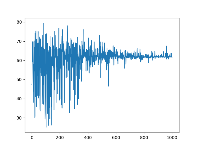
This will start the Vertical FL training for 1000 rounds with 3 clients. Eventhough the number of rounds is quite high, this should only take a few seconds to run as the model is very small.
Explanations#
Vertical FL vs Horizontal FL#
Horizontal Federated Learning (HFL or just FL) |
Vertical Federated Learning (VFL) |
|
|---|---|---|
Data Distribution |
Clients have different data instances but share the same feature space. Think of different hospitals having different patients’ data (samples) but recording the same types of information (features). |
Each client holds different features for the same instances. Imagine different institutions holding various tests or measurements for the same group of patients. |
Model Training |
Each client trains a model on their local data, which contains all the feature columns for its samples. |
Clients train models on their respective features without having access to the complete feature set. Each model only sees a vertical slice of the data (hence the name ‘Vertical’). |
Aggregation |
The server aggregates these local models by averaging the parameters or gradients to update a global model. |
The server aggregates the updates such as gradients or parameters, which are then used to update the global model. However, since each client sees only a part of the features, the server typically has a more complex role, sometimes needing to coordinate more sophisticated aggregation strategies that may involve secure multi-party computation techniques. |
Privacy Consideration |
The raw data stays on the client’s side, only model updates are shared, which helps in maintaining privacy. |
VFL is designed to ensure that no participant can access the complete feature set of any sample, thereby preserving the privacy of data. |
HFL |
VFL |
|---|---|
|
|
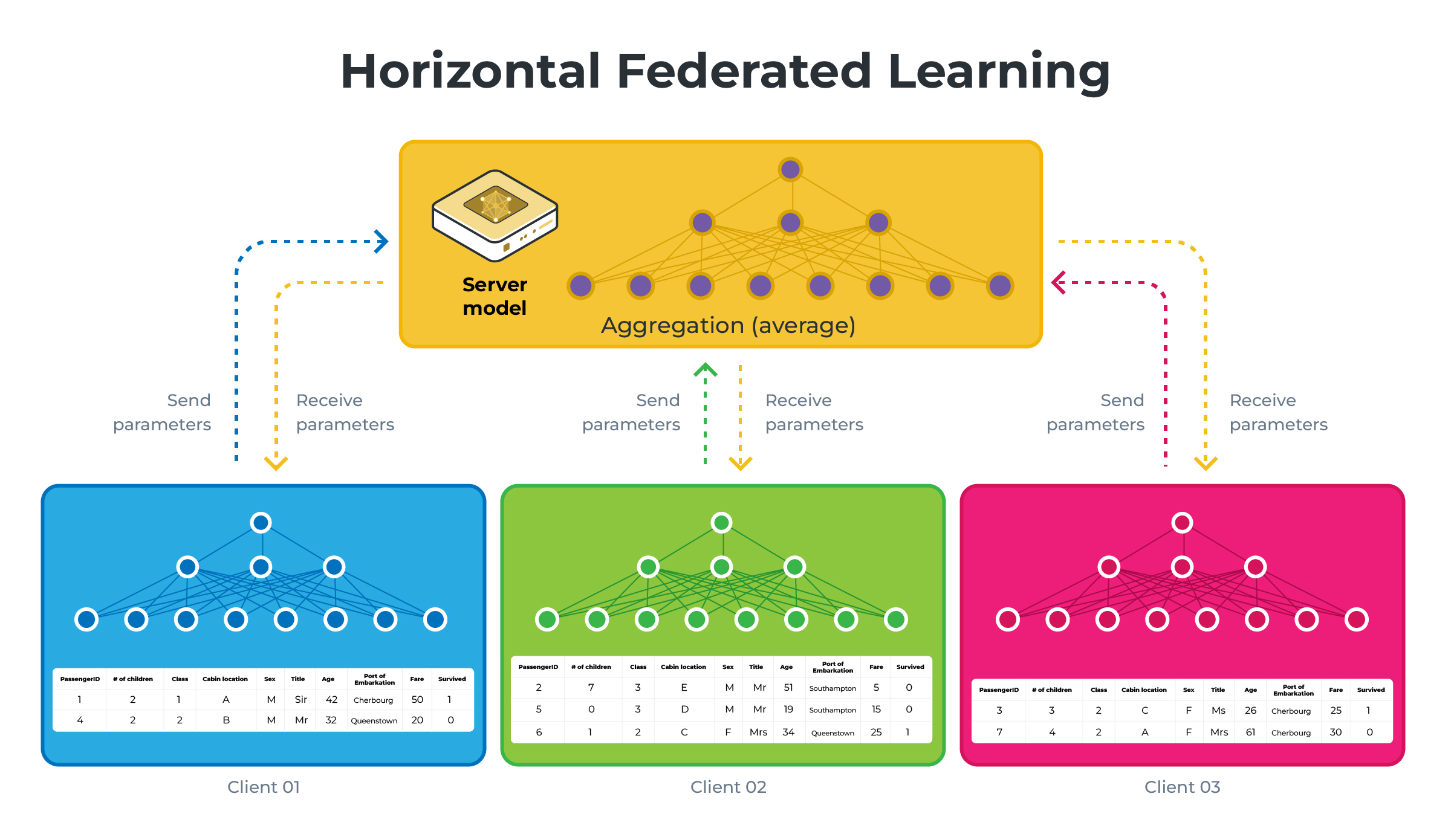
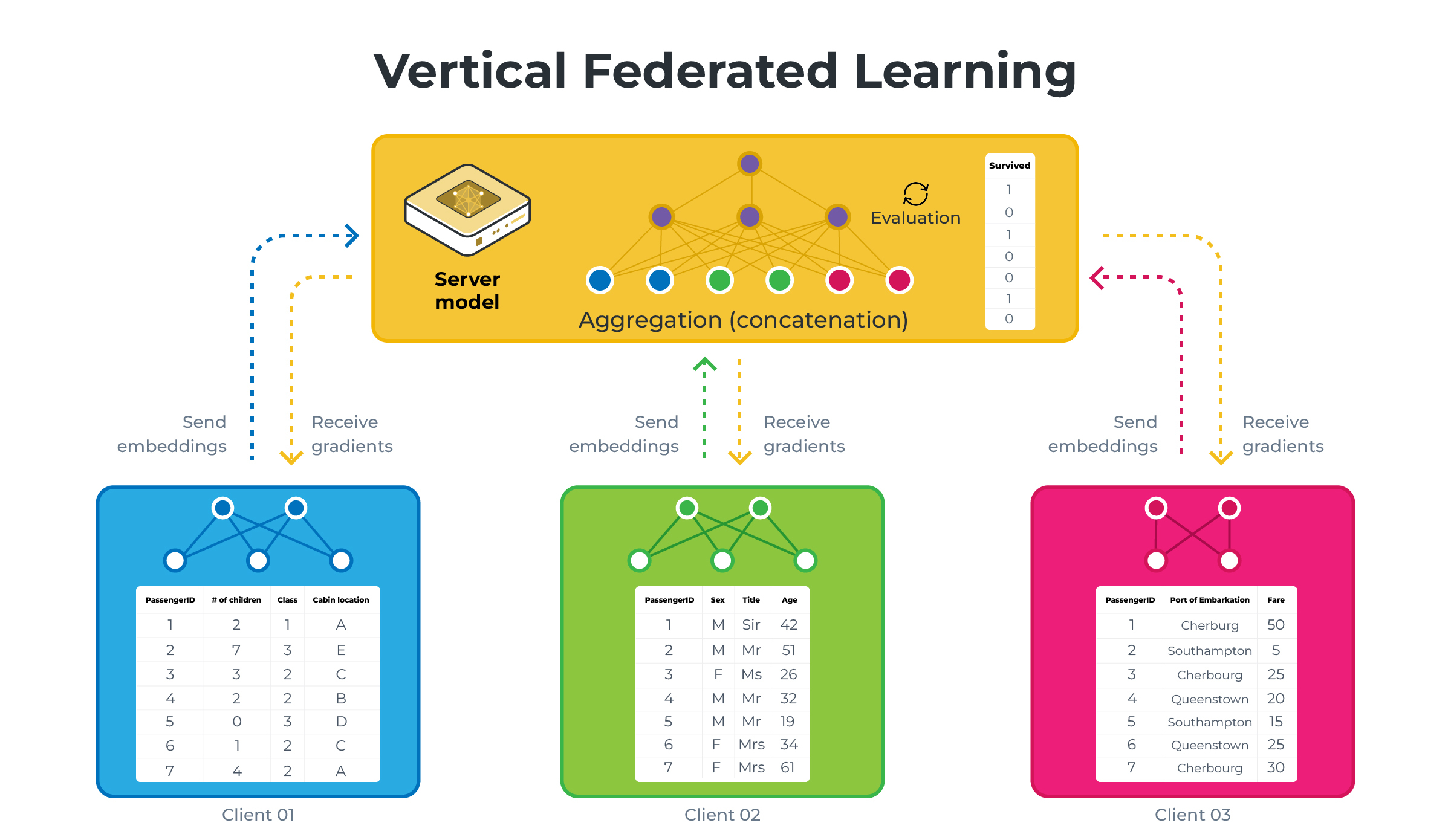
Those diagrams illustrate HFL vs VFL using a simplified version of what we will be building in this example. Note that on the VFL side, the server holds the labels (the Survived column) and will be the only one capable of performing evaluation.
Data#
About#
The Titanic Survival dataset is a popular dataset used to predict passenger survival on the Titanic based on various features.
You can see an exhaustive list of the features over on Kaggle.
The data is stored as a CSV file in _static/data/train.csv, it contains 892
samples with labels.
Preprocessing#
In task.py, you’ll find the preprocessing functions we’ll apply to our data:
Passengers are grouped by age: ‘Child’ for 10 years and under, ‘Adult’ for ages between 11 and 40, and ‘Elderly’ for those over 40. If the age isn’t listed, we’ll label it as ‘Unknown’.
  def _bin_age(age_series):
      bins = [-np.inf, 10, 40, np.inf]
      labels = ["Child", "Adult", "Elderly"]
      return (
          pd.cut(age_series, bins=bins, labels=labels, right=True)
          .astype(str)
          .replace("nan", "Unknown")
      )
We pull out titles from passengers’ names to help our model understand social status and family roles, simplifying rare titles into a single ‘Rare’ category and converting any French titles to their English equivalents.
  def _extract_title(name_series):
      titles = name_series.str.extract(" ([A-Za-z]+)\.", expand=False)
      rare_titles = {
          "Lady",
          "Countess",
          "Capt",
          "Col",
          "Don",
          "Dr",
          "Major",
          "Rev",
          "Sir",
          "Jonkheer",
          "Dona",
      }
      titles = titles.replace(list(rare_titles), "Rare")
      titles = titles.replace({"Mlle": "Miss", "Ms": "Miss", "Mme": "Mrs"})
      return titles
The first letter of each cabin number is used to identify the cabin area, with any missing entries marked as ‘Unknown’. This could provide insight into the passenger’s location on the ship.
We remove features like ‘PassengerId’, ‘Name’, and ‘Ticket’ that won’t be necessary for our model’s predictions.
Lastly, we convert categorical data points such as ‘Sex’, ‘Pclass’, ‘Embarked’, ‘Title’, ‘Cabin’, and the binned ‘Age’ into One-Hot encodings.
  def _create_features(df):
      # Convert 'Age' to numeric, coercing errors to NaN
      df["Age"] = pd.to_numeric(df["Age"], errors="coerce")
      df["Age"] = _bin_age(df["Age"])
      df["Cabin"] = df["Cabin"].str[0].fillna("Unknown")
      df["Title"] = _extract_title(df["Name"])
      df.drop(columns=["PassengerId", "Name", "Ticket"], inplace=True)
      all_keywords = set(df.columns)
      df = pd.get_dummies(
          df, columns=["Sex", "Pclass", "Embarked", "Title", "Cabin", "Age"]
      )
      return df, all_keywords
Partitioning#
In task.py, we also partition our data for our 3 clients to mirror real-life
collaborations where different organizations hold different feature sets:
def _partition_data(df, all_keywords):
    partitions = []
    keywords_sets = [{"Parch", "Cabin", "Pclass"}, {"Sex", "Title"}]
    keywords_sets.append(all_keywords - keywords_sets[0] - keywords_sets[1])

    for keywords in keywords_sets:
        partitions.append(
            df[
                list(
                    {
                        col
                        for col in df.columns
                        for kw in keywords
                        if kw in col or "Survived" in col
                    }
                )
            ]
        )

    return partitions
Client 1: This client looks at family connections and accommodations, working with features like the number of parents and children each passenger had on board (‘Parch’), the cabin number (‘Cabin’), and the ticket class (‘Pclass’).
Client 2: Here, the focus is on personal attributes. This client examines the passengers’ gender (‘Sex’) and societal roles as indicated by their titles (‘Title’).
Client 3: The final client handles the rest of the data that the first two don’t see. This includes the remaining features that give a broader view of the passengers’ information.
Each client is going to train their models on their own unique data without any idea of the passengers’ survival outcomes, which we’re trying to predict.
Once all clients have done their part, we combine their insights to form a comprehensive understanding, just as if different organizations were pooling their knowledge while keeping their data private. This is the essence of Vertical Federated Learning: separate but together, each contributing to a collective intelligence without sharing sensitive information.
Note that our final data processing function looks like that:
def get_partitions_and_label():
    df = pd.read_csv("_static/data/train.csv")
    processed_df = df.dropna(subset=["Embarked", "Fare"]).copy()
    processed_df, all_keywords = _create_features(processed_df)
    raw_partitions = _partition_data(processed_df, all_keywords)

    partitions = []
    for partition in raw_partitions:
        partitions.append(partition.drop("Survived", axis=1))
    return partitions, processed_df["Survived"].values
This returns the 3 partitions for our clients and the labels for our server.
Models#
Clients#
Each client’s model is a neural network designed to operate on a distinct subset of features held by a client. In this example we will use simple linear regression models.
class ClientModel(nn.Module):
    def __init__(self, input_size):
        super(ClientModel, self).__init__()
        self.fc = nn.Linear(input_size, 4)

    def forward(self, x):
        return self.fc(x)
The input_size corresponds to the number of features each client has, and this
model maps those features to a 4-dimensional latent space. The outputs are
essentially feature embeddings that capture the patterns within each client’s
data slice. These embeddings are then ready to be sent to the server for further
processing.
Server#
The server’s model acts as the central aggregator in the VFL system. It’s also a neural network but with a slightly different architecture tailored to its role in aggregating the client models’ outputs.
class ServerModel(nn.Module):
    def __init__(self):
        super(ServerModel, self).__init__()
        self.fc = nn.Linear(12, 1)
        self.sigmoid = nn.Sigmoid()

    def forward(self, x):
        x = self.fc(x)
        return self.sigmoid(x)
It comprises a single linear layer that accepts the concatenated outputs from
all client models as its input. The number of inputs to this layer equals the
total number of outputs from the client models (3 x 4 = 12). After processing
these inputs, the linear layer’s output is passed through a sigmoid activation
function (nn.Sigmoid()), which maps the result to a (0, 1) range, providing
a probability score indicative of the likelihood of survival.
Strategy#
The strategy we will write to perform the aggregation will inherit from FedAvg
and set the following additional attributes:
self.model = ServerModel(12)
self.initial_parameters = ndarrays_to_parameters(
    [val.cpu().numpy() for _, val in self.model.state_dict().items()]
)
self.optimizer = optim.SGD(self.model.parameters(), lr=0.01)
self.criterion = nn.BCELoss()
self.label = torch.tensor(labels).float().unsqueeze(1)
With labels given as an argument to the strategy.
We then redefine the aggregate_fit method:
def aggregate_fit(
    self,
    rnd,
    results,
    failures,
):
    # Do not aggregate if there are failures and failures are not accepted
    if not self.accept_failures and failures:
        return None, {}

    # Convert results
    embedding_results = [
        torch.from_numpy(parameters_to_ndarrays(fit_res.parameters)[0])
        for _, fit_res in results
    ]
    embeddings_aggregated = torch.cat(embedding_results, dim=1)
    embedding_server = embeddings_aggregated.detach().requires_grad_()
    output = self.model(embedding_server)
    loss = self.criterion(output, self.label)
    loss.backward()

    self.optimizer.step()
    self.optimizer.zero_grad()

    grads = embedding_server.grad.split([4, 4, 4], dim=1)
    np_grads = [grad.numpy() for grad in grads]
    parameters_aggregated = ndarrays_to_parameters(np_grads)

    with torch.no_grad():
        correct = 0
        output = self.model(embedding_server)
        predicted = (output > 0.5).float()

        correct += (predicted == self.label).sum().item()

        accuracy = correct / len(self.label) * 100

    metrics_aggregated = {"accuracy": accuracy}

    return parameters_aggregated, metrics_aggregated
This is where all the magic happens. We first convert the np.arrays that we
received from our clients to tensors, before concatenating the 3 embeddings
together. This means that we go from 3 tensors of size (892, 4) to 1 tensor of
size (892, 12). The combined embeddings are fed through the server model to
get the prediction output. The loss between the predicted output and the actual
labels is calculated. Backward propagation is then performed to calculate the
gradients, which are used to update the server model’s parameters.
The optimizer updates the server model’s parameters based on the calculated gradients, and the gradients are reset to zero to prepare for the next round of aggregation.
The gradients from the server model’s embedding layer are then split according to the size of the output from each client model (assuming equal size for simplicity here), ready to be sent back to the respective client models.
Finally, with no gradient calculation needed, the model’s predictions are compared to the true labels to calculate the accuracy of the model after the update.
Note that this aggregate_fit function returns gradients instead of trained
weights. This is because, in this setting, sharing gradients allows each
participant to benefit from the collective feedback gathered from the entire
pool of data without the need to align their different feature spaces (trained
weights are directly tied to specific features of the dataset but not gradients,
which are just a measure of the sensitivity of the loss function to changes in
the model’s parameters). This shared feedback, encapsulated in the gradients,
guides each participant’s model to adjust and improve, achieving optimization
not just based on its own data but also leveraging insights from the entire
network’s data.
We do not need to return parameters here because updates are completed locally
in VFL. But the server should still send the gradients back to all clients to
let them continue the back prop and update their local model. In Flower, the
parameters returned by aggregate_fit will be stored and sent to
Client.evaluate via configure_fit. So we take advantage of this and return
our gradients in aggregate_fit so that they’ll be sent to Client.evaluate as
parameters. That’s also why we can obtain gradients from the parameters
argument in Client.evaluate (see next section).
The last thing we have to do is to redefine the aggregate_evaluate function to
disable distributed evaluation (as the clients do not hold any labels to test
their local models).
def aggregate_evaluate(
    self,
    rnd,
    results,
    failures,
):
    return None, {}
Client class and function#
Our FlowerClient class is going to be quite straight forward.
class FlowerClient(fl.client.NumPyClient):
    def __init__(self, cid, data):
        self.cid = cid
        self.train = torch.tensor(StandardScaler().fit_transform(data)).float()
        self.model = ClientModel(input_size=self.train.shape[1])
        self.optimizer = torch.optim.SGD(self.model.parameters(), lr=0.01)
        self.embedding = self.model(self.train)

    def get_parameters(self, config):
        pass

    def fit(self, parameters, config):
        self.embedding = self.model(self.train)
        return [self.embedding.detach().numpy()], 1, {}

    def evaluate(self, parameters, config):
        self.model.zero_grad()
        self.embedding.backward(torch.from_numpy(parameters[int(self.cid)]))
        self.optimizer.step()
        return None
After defining our model and data attributes (respectively self.model and
self.train), we define our fit function as such: the self.model(self.train)
performs a forward pass using the client’s local training data (self.train).
This generates the embeddings (feature representations) for the data. To conform
with the return type of the fit function, we need to return a list of
np.arrays (hence the conversion), the number of samples, which won’t be used
on the server side, so we just return 1, and then an empty dict.
For the evaluate function, we perform our model’s backward pass using the
gradients sent by the server and then update our local model’s parameters based
on those new gradients. Note that the loss and num_examples we return in our
evaluate function are bogus, as they won’t be used on the server side.
The client_fn we will use in our start_simulation function to generate our 3
clients will be very basic:
partitions, label = get_partitions_and_label()

def client_fn(cid):
    return FlowerClient(cid, partitions[int(cid)]).to_client()
We pass a client_id and its corresponding partition to each client.
Evaluation#
Please note that we do not perform distributed evaluation. This is because only the server holds some labels to compare the results to. This is why the only evaluation we perform is on the server side.
In this example, we use the FlowerClient evaluate function for
backpropagation instead of using it for evaluation. We do this because we know
that the evaluate function of the clients will be called after the fit
function. This allows us to aggregate our models in aggregate_fit and then
send them back to the clients using this evaluate function and perform the
backpropagation. This is not done for evaluation, hence why we return None in
the aggregate_evaluate function of the strategy.
Starting the simulation#
Putting everything together, to start our simulation we use the following function:
hist = fl.simulation.start_simulation(
    client_fn=client_fn,
    num_clients=3,
    config=fl.server.ServerConfig(num_rounds=1000),
    strategy=Strategy(label),
)
As mentioned before, we train for 1000 rounds but it should still last only a few seconds.
Note that we store the results of the simulation into hist, this will allow us
to use the plot.py file to plot the accuracy as a function of the number of
rounds.
Results#
Here we can observe the results after 1000 rounds: